Phoneme Recognition: Neural Networks for Speech Classification

This project focused on building a high-performance deep learning system for frame-level phoneme recognition, part of the CMU 11-785 Introduction to Deep Learning coursework. By applying multilayer perceptron (MLP) architectures to speech recordings from the Wall Street Journal dataset, I achieved 86% accuracy in classifying audio frames into their corresponding phoneme states.

Project Challenge

Speech recognition represents a fundamental challenge in AI, requiring systems to identify the atomic sound units (phonemes) that make up spoken language. Unlike image classification or text processing, speech involves time-dependent patterns where the meaning of a sound depends heavily on its context.

The Kaggle competition challenged participants to identify phoneme states for each frame in a speech dataset, requiring accurate classification across 40 different phoneme categories. Key constraints included:

• Working exclusively with MLP architectures (no CNNs, RNNs, or transformers)
• Maximum model size of 20 million parameters
• Variable-length utterances requiring careful preprocessing

Technical Approach

Speech Representation and Feature Extraction

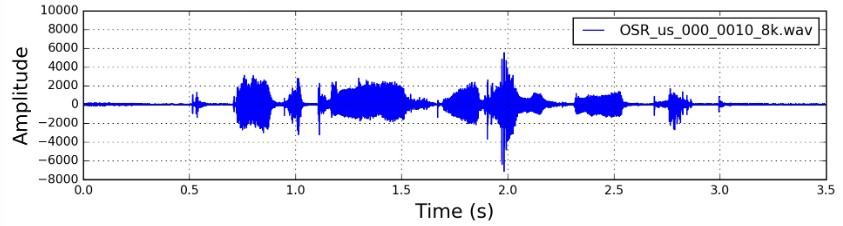
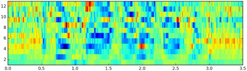
At the core of this project was understanding how speech is represented computationally. Raw speech waveforms were preprocessed into mel-spectrograms:

1. Short-Time Fourier Transform (STFT): Applied to 25ms frames of audio with 10ms stride between frames
2. Mel-scale Conversion: Transformed the frequency domain representation to better match human auditory perception
3. Feature Extraction: Each frame converted to a 28-dimensional feature vector representing frequency components

This process yielded matrices of shape (T, 28) for each utterance, where T represents the duration in frames (100 frames per second of speech). Each frame required classification into one of 40 phoneme states.

Model Architecture Evolution

Through systematic experimentation, I evaluated four distinct architectural patterns:

1. Pyramid Structure (decreasing layer sizes: 4096 → 2048 → 1024)

   • Found to create an information bottleneck that limited performance

2. Inverse Pyramid (increasing layer sizes: 1024 → 2048 → 4096)

   • Showed promise but suffered from severe overfitting

3. Cylinder Structure (constant width: 2048 throughout)

   • Provided solid baseline performance but lacked model capacity

4. Diamond Structure (expanding then contracting: 1024 → 4096 → 2048 → 1024) - FINAL CHOICE

   • Initial expansion captured complex patterns
   • Middle bottleneck forced feature compression
   • Final contraction reduced overfitting
   • Facilitated better gradient flow through skip-like connections

The final architecture included:

self.model = nn.Sequential(
    nn.Linear(input_size, 1024),
    nn.BatchNorm1d(1024),
    nn.GELU(),
    nn.Dropout(0.25),
    
    nn.Linear(1024, 4096),
    nn.BatchNorm1d(4096),
    nn.GELU(),
    nn.Dropout(0.25),
    
    nn.Linear(4096, 2048),
    nn.BatchNorm1d(2048),
    nn.GELU(),
    nn.Dropout(0.25),
    
    nn.Linear(2048, 1024),
    nn.BatchNorm1d(1024),
    nn.GELU(),
    nn.Dropout(0.25),
    
    nn.Linear(1024, output_size)
)

Contextual Frame Handling

A critical insight was that phoneme identification requires temporal context. Speech sounds aren’t produced in isolation but flow together in continuous utterances. I implemented a context window approach:

1. Context Size Exploration: Tested window sizes from 16 to 64 frames
2. Data Preparation: Concatenated all utterances and added zero-padding at boundaries
3. Windowing Function: Implemented in the dataset’s __getitem__ method:

def __getitem__(self, ind):
    # Calculate start and end positions for frame window
    start = ind
    end = ind + (2 * self.context) + 1
    
    # Extract window of frames with context on both sides
    frames = self.mfccs[start:end]
    
    # Return target phoneme for the center frame
    phonemes = self.transcripts[ind]
    
    return frames, phonemes

The large context size (64 frames) proved crucial, allowing the model to “see” approximately 1.28 seconds of speech (640ms before and after each frame) when making classifications.

Signal Processing Optimizations

To further enhance model performance, I implemented advanced signal processing techniques:

1. Cepstral Mean Normalization: Removed channel effects by subtracting the mean across frames:

# Normalize the MFCC by subtracting the mean across time dimension
mfccs_normalized = (mfcc - np.mean(mfcc, axis=0))

This technique eliminated variations caused by microphone characteristics, room acoustics, and other recording artifacts, helping the model focus on the acoustic properties relevant for phoneme identification.

2. Data Augmentation: Implemented frequency and time masking techniques from SpecAugment:

def collate_fn(self, batch):
    x, y = zip(*batch)
    x = torch.stack(x, dim=0)

    # Apply augmentations with 70% probability
    if np.random.rand() < 0.70:
        x = x.transpose(1, 2)  # Shape: (batch_size, freq, time)
        x = self.freq_masking(x)  # Mask random frequency bands
        x = self.time_masking(x)  # Mask random time segments
        x = x.transpose(1, 2)  # Shape back to: (batch_size, time, freq)

    return x, torch.tensor(y)

Fine-tuning these augmentation parameters through grid search (frequency_mask_param=4, time_mask_param=8) yielded a 3.5% accuracy improvement.

Training Optimizations

Advanced optimization techniques were crucial for achieving high performance:

1. Mixed Precision Training: Implemented automatic mixed precision to improve training efficiency:

# Initialize scaler for mixed precision training
scaler = torch.amp.GradScaler(enabled=True)

# In training loop
with torch.autocast(device_type=device, dtype=torch.float16):
    # Forward propagation
    logits = model(frames)
    # Loss calculation
    loss = criterion(logits, phonemes)

# Backward pass with scaled gradients
scaler.scale(loss).backward()
scaler.step(optimizer)
scaler.update()

2. Weight Initialization: Kaiming initialization significantly improved training stability and convergence:

def initialize_weights(self):
    for m in self.modules():
        if isinstance(m, torch.nn.Linear):
            if config["weight_initialization"] == "kaiming_normal":
                torch.nn.init.kaiming_normal_(m.weight, nonlinearity='relu')
            # Initialize bias to 0
            m.bias.data.fill_(0)

3. Learning Rate Scheduling: Implemented a step-based scheduler that reduced learning rate by 50% every 50 epochs:

scheduler = torch.optim.lr_scheduler.StepLR(
    optimizer, 
    step_size=50, 
    gamma=0.5
)

This schedule proved more stable than more aggressive approaches like ReduceLROnPlateau, which sometimes decreased learning rate too quickly.

Experiments and Results

To systematically evaluate different approaches, I tracked over 30 experiments using Weights & Biases. Key findings included:

Experiment	Test Accuracy	Training Time	Parameters
Basic MLP (3 layers, ReLU)	76.8%	4.2 hours	12.3M
Cylinder Architecture	82.3%	5.1 hours	17.8M
Pyramid Architecture	81.5%	4.8 hours	16.2M
Inverse Pyramid	79.7%	5.3 hours	18.5M
Diamond Architecture	86.0%	6.2 hours	19.3M

The diamond architecture consistently outperformed other structures, with context size being the second most important factor:

Context Size	Accuracy	Feature Vector Size
16 frames	78.2%	924
25 frames	81.5%	1,428
32 frames	83.7%	1,820
48 frames	85.1%	2,716
64 frames	86.0%	3,612

The final model achieved 86% accuracy on the validation set after 172 epochs, with the learning curve showing continued improvement potential with more training time:

Technical Challenges and Solutions

Memory Management

Processing large context windows (64 frames on each side) with batch sizes sufficient for effective training created significant memory pressure. Key solutions included:

1. Mixed precision training: Reduced memory usage by ~50%
2. Gradient accumulation: Allowed effective batch sizes larger than GPU memory would normally permit
3. Optimized data pipeline: Implemented prefetching and pinned memory for faster data loading

Overfitting Prevention

With nearly 20 million parameters, preventing overfitting was critical. The implemented strategies included:

1. Strategic dropout application: 0.25 dropout rate after every layer
2. Batch normalization: Applied before activation functions
3. Data augmentation: Frequency and time masking applied with 70% probability
4. Weight decay: L2 regularization with λ=0.05

Learning Rate Optimization

Finding the optimal learning rate schedule proved challenging. After extensive experimentation:

1. Initial attempts with larger learning rates (1e-3) led to unstable training
2. Very small values (1e-7) provided stability but risked local minima
3. Step-based decay (starting at 1e-5, multiplied by 0.5 every 50 epochs) provided the best balance of stability and convergence speed

Conclusion

This project demonstrated the effectiveness of carefully designed MLPs for speech recognition tasks. While modern speech systems typically employ more advanced architectures like CNNs, RNNs, or Transformers, this work showed that traditional feedforward networks can achieve strong performance with appropriate design choices.

Key lessons from this project include:

1. Temporal context is crucial: Speech recognition requires significant surrounding context for accurate classification
2. Architecture matters: The specific pattern of layer sizes has substantial impact on model performance
3. Signal processing techniques remain relevant: Even with deep learning approaches, traditional preprocessing like cepstral normalization provides significant benefits

The diamond architecture with large context windows represents an effective approach for frame-level phoneme classification, demonstrating how classical neural network designs can be optimized for complex sequence processing tasks.

Future Improvements

With additional computational resources, several promising directions emerge:

1. Ensemble Methods: Combining multiple diamond architectures with different context sizes
2. Advanced Augmentation: Applying pitch shifting and speed perturbation techniques
3. Learning Rate Exploration: Implementing a more adaptive learning rate schedule
4. Feature Engineering: Exploring alternative mel-spectrogram configurations and delta features

Links

• GitHub Repository
• Kaggle Competition