I took 16-720 in the fall of 2024. It covers image formation, camera geometry and calibration, multi-view geometry, stereo, 3D reconstruction, motion analysis, physics-based vision, segmentation and recognition. That is a lot of territory for one semester, and the way it gets covered is blunt: the course description says evaluation is based on homeworks, and it means it. Five of them.
Everything below comes out of my own write-ups and result files, so the numbers are the ones I actually got, including the bad ones.
Bag of Visual Words, and Tuning That Refuses to Go Straight
The first homework is scene recognition on eight classes: aquarium, desert, highway, kitchen, laundromat, park, waterfall and windmill, fifty test images each. You build a filter bank of Gaussians, derivatives of Gaussian in x and y, and Laplacians of Gaussian at several scales, run k-means over the responses to build a dictionary of visual words, convert each image to a spatial pyramid of word histograms, and classify by nearest neighbour under histogram intersection.
With the handout defaults, K equal to 10 words and L equal to 1, I got 54.25 percent. Then I tuned, and the tuning did not behave the way I expected. K at 30 and L at 3 with scales of 1, 2 and 4 gave 56 percent. L at 4 gave 60 percent. K at 65 gave 61.75 percent. Alpha at 55, K at 65, L at 4 and scales of 1, 2, 3 and 4 gave 62.75 percent. And then it stopped. Whatever I changed, the accuracy sat around 60 percent.
So I threw the tuned configuration away, went back to the starting parameters, and raised the dictionary to 100 words. That gave 67 percent, and it is what is still in my opts.py and my accuracy.txt. Dictionary size was doing almost all of the work. The pyramid depth I had spent hours on was noise dressed up as progress.
The more useful thing was watching where the errors sat. At the default settings the aquarium wordmaps looked like waterfall wordmaps, and aquarium images were among the ones read that way. The worst class at those settings was not aquarium, though. It was laundromat, at 16 correct out of 50, with 21 of its images called kitchen.

That is an aquarium the classifier got wrong, drawn as visual words. Almost nothing in it is aquarium-specific. It is a few large flat regions and two vertical bands, which is also a perfectly good description of falling water.
By the final configuration one of those two failures had moved and the other had not. My confusion matrix at 67 percent has aquarium at 42 out of 50, the best class in the set, up from 30 at the defaults. Laundromat is still the worst, at 23 out of 50, with 16 of its images still called kitchen. Raising the dictionary lifted aquarium by twelve images and barely touched the laundromat and kitchen pair, which was the dominant error before the tuning and after it. Both of those are boxy interiors full of white rectangular appliances, and a bigger vocabulary of texture words was never going to separate them, because the thing that separates them is not texture. That is the split I now look for: errors that come from a representation being too coarse, which tuning can reach, and errors that come from the representation not encoding the distinction at all, which it cannot.
Two Parameters Decide Whether Matching Works At All
The second homework is planar homographies. You derive the direct linear transform constraint, prove the pure-rotation case and show that squaring the homography corresponds to rotating by twice the angle, then implement matching with a FAST corner detector and BRIEF descriptors compared by Hamming distance, normalised homography estimation, RANSAC, and the augmented reality bit where you warp a book cover onto a photo of a different book on a desk.
The part I remember is the ablation. Two knobs: sigma, the FAST corner threshold, and ratio, the nearest-neighbour ratio test. I swept sigma over 0.05, 0.15, 0.30, 0.45 and 0.60, and ratio over 0.3, 0.5, 0.7 and 0.9, matching the Computer Vision: A Modern Approach cover against a photo of it on a desk.
At sigma 0.15 and ratio 0.7 you get maybe two dozen correspondences, most of them landing where they should. Change only the ratio to 0.9 and you get this.
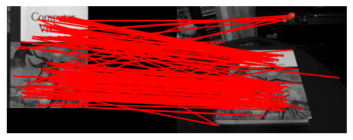
Same detector, same descriptor, same two images, one number changed. It is easy to look at that and think the matcher is broken. It is not. It is doing exactly what it was told, which was to accept a match even when the second-best candidate was almost as good.
That homework is where I stopped trusting a pipeline just because it ran.
BRIEF Does Not Survive Rotation, and It Is Not Subtle
The same homework asks you to write briefRot: rotate the cover image in ten degree steps through a full turn, count matches at each angle, and plot the result on a log axis.
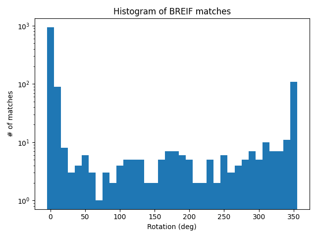
About a thousand matches at zero degrees. Roughly ninety at ten. By twenty degrees it is in the single digits, and it stays there for most of the circle before climbing back near 350. An order of magnitude lost in the first ten degrees, and two by twenty, because BRIEF samples fixed pixel pairs in a fixed orientation, and the binary string is not the same string once you turn the patch.
You can read that BRIEF is not rotation invariant in a sentence. Generating this plot with your own descriptor is a different kind of knowing. It is also where I first understood why deployed vision systems care so much about controlling camera pose instead of asking the algorithm to be heroic.
Reconstruction Is Mostly Careful Bookkeeping
Homework three is 3D reconstruction on the temple image pair: normalised eight point algorithm for the fundamental matrix, singularity enforcement, essential matrix from the intrinsics, triangulation, then choosing the correct camera among the four candidate extrinsics by checking that points land in front of both cameras and keeping the lowest reprojection error. After that, epipolar correspondence with a Gaussian-weighted patch, a point cloud of the temple, RANSAC over noisy correspondences, and bundle adjustment.
The number I still think about is from the bundle adjustment on the noisy correspondences. In the run I submitted, the reprojection objective went from 80,328,527.99 before to 11.33 after. Another run of the same notebook in that folder starts at 352.84 and ends at 10.89. The ending value is stable across both. The starting value moves by more than five orders of magnitude depending on what the initialisation happened to be, and that spread is the actual lesson.
That gap is not a triumph of optimisation. It is what happens when your initialisation is bad and your optimiser is fine. Almost none of geometric vision is clever. It is coordinate conventions, homogeneous divisions, which matrix goes on which side, and whether you remembered to normalise. Every bug I had in that homework was a bookkeeping bug.
Writing Backpropagation Out By Hand
Homework four makes you build a fully connected network in numpy with nothing underneath it: weight initialisation, sigmoid and softmax forward passes, cross entropy, the backward pass, and a stochastic gradient descent loop over random batches. Then you train it on NIST36, thirty-six classes of upper case letters and digits, with one hidden layer of 64 units, batch size 64, learning rate 3e-3, for 50 epochs.
Training accuracy reached 0.92 by the last logged epoch. Validation came out at 74.56 percent and test at 74.39 percent. The handout asked for 75 percent. I did not get there, and my write-up says so.
The learning rate sweep afterwards taught me more. Same network, same data, same fifty epochs, three rates. At ten times the tuned rate, 3e-2, test accuracy was 52.11 percent. At one tenth, 3e-4, it was 65.72 percent. At the tuned 3e-3, it was 75 percent, slightly ahead of my main run on a different random seed, which changes both the initialisation and the batch draw. Being ten times too fast cost me more than being ten times too slow, which is not what my intuition said at the time. Too slow is a network that has not finished. Too fast is a network that is bouncing.
The second half hands you a pretrained Faster R-CNN and a car video, and asks you to build a tracker by linking detections across frames with an intersection over union rule. That was the first thing I wrote that had to hold an identity across time, and it was the harder half.
Photometric Stereo, and a Rank That Was Not Three
The photometric stereo homework starts out calibrated and Lambertian. Render a sphere under a known light, stack seven images into an intensity matrix, solve least squares for the pseudonormals, recover albedo and normal maps, then integrate the normals into a surface with the Frankot-Chellappa algorithm.
Under the Lambertian model that intensity matrix should have rank 3, because there are three degrees of freedom in a surface normal scaled by albedo. Mine had singular values of 79.36, 13.16, 9.22, 2.41, 1.62, 1.26 and 0.89. That is rank 7. There is a steep drop after the first value and another after the third, but nothing goes to zero.
Writing up why is the most valuable paragraph I produced in that course. The theory is not wrong. It describes an ideal Lambertian surface under ideal point lights with no noise, and I had none of those three. Noise, rendering artefacts and non-ideal light directions all push energy into the trailing singular values. The uncalibrated half of the assignment leans on exactly that structure, truncating to the top three singular values and then hunting for the transform that makes the field integrable.
A Year Later, Scoring Somebody Else’s Detector
I hit computer vision again in 24-784, a course on trustworthy AI, where the first challenge was not building a detector but evaluating one. Stop sign detections on SafeBench_v2, 1,636 predicted boxes, 66 of them stop signs, against 92 ground truth stop signs. We implemented intersection over union from the box corners and average precision the COCO way, with a monotonic precision envelope and 101 point interpolation.
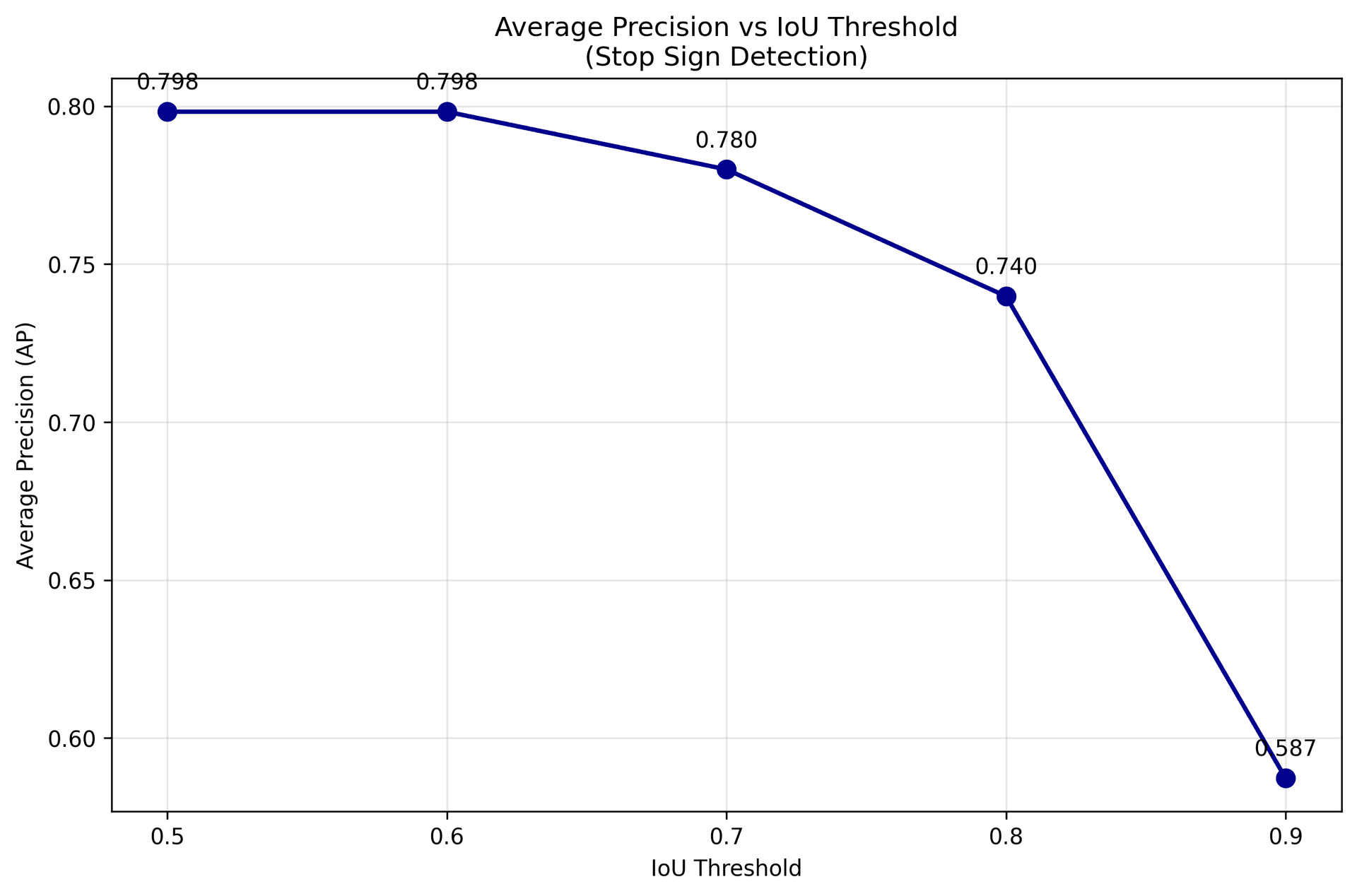
AP is 0.798 at IoU 0.5 and unchanged at 0.6. It slips to 0.780 at 0.7, 0.740 at 0.8, and then falls to 0.587 at 0.9. The mean over that range is 0.741. One thing we flagged in the report and never resolved: the assignment said to expect AP somewhere in the 0.3 to 0.5 range, and we came out well above it, which means either the model was better than the handout assumed or we were scoring a different evaluation scenario than the one that range was written for.
The shape is the part I trust, and it is the whole lesson. A model that looks like it has a 0.80 detection problem actually has a localisation problem, and it only becomes visible when you demand tighter boxes. If somebody quotes a single AP number without the threshold attached, they have told you almost nothing. The gap between the flat part of that curve and the cliff is the gap between knowing a stop sign is present and knowing where it is.
What Carried Over
I now work on a vision system that measures fish, and the parts of 16-720 that show up in my week are not the parts I expected. Not the architectures. The calibration.
Every frame we capture carries its own scale reference, the calibrated mat and AprilTag I described in the autonomy post, because homework two taught me that geometry you cannot re-derive from the image itself is geometry you are trusting a tripod to preserve. The rotation histogram taught me to control the camera rather than argue with the descriptor.
And the confusion matrix from homework one taught me the habit I use most: look at which class is losing, and to whom. A model that confuses laundromats with kitchens is telling you something real about your features. A single accuracy number is telling you nothing at all.